

Overlap rate of neighboring ommatidia
The compound eye camera structure is designed in a way that naturally results in some degree of overlap in the field of view between neighboring ommatidia. By determining the ommatidium-axis angle, we can ensure that this overlap rate tends towards a fixed value. We conducted a statistical analysis of the overlap rate between all neighboring ommatidia for the proposed compound eye structure, and the results are presented in Table 2. Our compound eye spherical shell structure comprises 61 ommatidia arranged radially from the center of the spherical shell. These ommatidia are organized in a 5-layer structure. We have calculated the overlap rate between the ommatidia in two categories: overlap across layers and overlap between ommatidia of the same layer. Figure 4c–e demonstrates that the angle of the ommatidium axial pinch is fixed, and its overlap rate stabilizes. The overlapping region of the field of view ensures that no part of the field of view is omitted, resulting in improved energy reception and subsequently enhancing the SNR of the system. Furthermore, it provides a matching benchmark for the reconstruction of the large field of view.
Theoretical observation field of view:
$$\beginaligned FOV_total = 2(n_total-1)\times \theta + 2\omega \endaligned$$
(1)
The overlap rate \(\eta\) of adjacent ommatidia is calculated as follows:
$$\beginaligned \eta = \fracsin(2\omega -\theta )2cos(\omega -\theta )sin\omega \endaligned$$
(2)
where \(\omega = 14^\circ\), the value of \(\theta\) is related to the position of ommatidia, n represents the layer of the ommatidium, with the central ommatidium being the first layer arranged radially. The value of \(n_total\) represents the number of eyes located at the equatorial position of the shell. Due to the central symmetry of the lens’s physical position, the 61 ommatidia can be classified into 8 spatial position relationships, divided into two categories. The first category includes the relationship between adjacent ommatidia in each layer except for the central ommatidium, and \(\theta\) for this category can be calculated using Eq. (3).The second category can be summarized as the relationship between adjacent ommatidia across layers in terms of the angle of the optical axis. This includes the clear relationship between 9 ommatidia evenly distributed along the large circular arc of the spherical shell (\(\theta =10^\circ\)), as well as the relationships between special positions of ommatidia such as 2–5, 4–8, 5–8, 7–12, 8–12, and 8–13. See Fig. 4b for the numbering of ommatidia in the spherical shell. The optical axis angle of these specific positions is obtained through spatial calculations, which can calculate the overlap rate of the field of view, and the neighboring ommatidia optical axis angle equation (4) at specific positions is summarized according to the method of finding the vector angle.
The angle between adjacent ommatidia optical axes on the same layer:
$$\beginaligned \theta _n = arccos\bigg [1-sin^2(n-1)\theta \cdot \Big (1-cos\big (\frac\pi 3(n-1)\big )\Big )\bigg ], \quad n= 2,3,4,5 \endaligned$$
(3)
Adjacent layer special position ommatidia’s optical axis angle:
$$\beginaligned \beginaligned \theta _2-5&= arccos(cos2\theta cos\theta + cos \frac\pi 6sin2\theta sin\theta ) \\ \theta _4-8&= arccos(cos3\theta cos2\theta + cos \frac\pi 9sin3\theta sin2\theta ) \\ \theta _5-8&= arccos(cos3\theta cos2\theta + cos \frac\pi 18sin3\theta sin2\theta ) \\ \theta _7-12&= arccos(cos4\theta cos3\theta + cos \frac\pi 12sin4\theta sin3\theta ) \\ \theta _8-12&= arccos(cos4\theta cos3\theta + cos \frac\pi 36sin4\theta sin3\theta ) \\ \theta _8-13&= arccos(cos4\theta cos3\theta + cos \frac\pi 18sin4\theta sin3\theta )\\ \endaligned \endaligned$$
(4)

Spherical shell ommatidium position distribution and its field of view overlap ratio. (a) Imaging schematic. (b) Spherical shell sub-lens array a confident schematic distribution. (c) Sub-lens overlap for an optical axis angle of \(10^\circ\). (d) Overlap ratio of adjacent sub-lenses in each layer. (e) Overlap ratio of adjacent sub-lenses across layers.
Energy correction based on compound eye optical system
We chose the Stirling-cooled mid-wave infrared detector because its energy response error is relatively small, even with ambient temperature changes and temperature drift. After conducting comprehensive tests on various correction algorithms, we selected a commonly used one-point correction and improved integration time adjustment based on the two-point correction algorithm. This was used in conjunction with eliminating the nonuniformity of the pixel response to eliminate the detector’s original image in the blind element. The principle is shown in Eqs. (5)–(8), where (i, j) in \(S_i,j\left( \phi \right)\)are the coordinates of the detector cells in the image array, \(g_i,j\left( \phi \right)\) is the pixel response rate, \(\Phi\) is the irradiance incident to the detector cells, \(o_i,j\left( \phi \right)\) is the dark current; and \(\phi _1\) is the calibration point to obtain the average difference \(D_i,j\) to compensate for the image element’s dark current. The basic two-point correction selects two radiance calibration points, \(\phi _L\) and \(\phi _H\) for correction. The experiments compare the non-uniform correction effects of one-point correction and integral time-adjusted two-point correction algorithms in various scenarios.
A one-point correction compensates for the dark current:
$$\beginaligned \overlineS(\phi _1)= & \frac1N \times M\sum _i=1^N\sum _j=1^MS_i,j(\phi _1) \endaligned$$
(5)
$$\beginaligned D_i,j= & S_i,j(\phi _1) – \overlineS(\phi _1) \endaligned$$
(6)
The two-point correction corrects the gain factor:
$$\beginaligned \overlineS_L= & \frac1N \times M\sum _i=1^N\sum _j=1^MS_i,j(\phi _L) \endaligned$$
(7)
$$\beginaligned \overlineS_H= & \frac1N \times M\sum _i=1^N\sum _j=1^MS_i,j(\phi _H) \endaligned$$
(8)
The straight lines determined by \((\phi _L,\overlineS_L)\) and \((\phi _H,\overlineS_H)\) is used as the calibration line, and the two-point calibration based on integration time takes into account the influence of different integration times on the detector’s pixel response curve. By collecting batches of data points at different response times, a better correction of the gain coefficient is achieved. The compound-eye camera system for a single detector with multiple apertures can perform the correction for all ommatidia simultaneously, and the correction results for different scenes are depicted in Fig. 5.
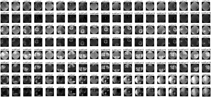
Comparison of calibration results for point light, single letter, multi-letter and scene images.

Gray-scale response of each ommatidium.
Experiments show that the generalized one-point and two-point correction algorithms are still insufficient for correcting compound eye images, see Fig. 6. Due to the special structure of the compound eye camera, the angle between the optical axis of the small lenses causes the outer ring of ommatidia to experience energy attenuation in their projection. Due to the small angle between the optical axis of the ommatidia, we will approximate attenuation as a linear function to compensate for the energy. \(I_true\) represents the true value of the grayscale image whereas \(I_redu\) represents the image’s attenuation. The enhancement coefficients use \(\tau\) and the equation is shown in (9):
$$\beginaligned I_true = \tau \cdot I_redu \endaligned$$
(9)
The calculation of \(\tau\) is based on statistical data obtained by analyzing a large number of experimental results, which compensates for the energy attenuation to a certain extent, but it is still necessary to further explore the energy correction method for the special compound eye camera structure.

Imaging results of infrared compound eye camera system. (a) Checkerboard target homemade. The red markings indicate the positions of checkerboards in the fifth layer of ommatidia. (b), (c) and (d) Imaging effect of target at different angles. (e) The outdoor imaging effect of a compound eye camera. The yellow markings indicate the position of ground containers, the green markings indicate the words of the building, and the blue markings represent rectangular buildings.
Figure 7 displays the laboratory and outdoor scene images that were directly captured. The panoramic image allows the ommatidia at the edge of the fifth circle to detect changes in optical flow of moving targets, but the image detail quality is poor. As previously mentioned, errors were encountered during manual assembly, and specific calibration methods for the spherical infrared camera were lacking, resulting in a progressive loss of energy in the compound eye camera’s ommatidia. The advantage of small edge distortions is evident in the compound eye structure camera. The distortion of ommatidia in the compound eye structure is significantly reduced under the same field of view, resulting in smaller edge distortions in the reconstructed image. The theoretical field of view range of the camera was tested by calibrating it on a parallel light pipe calibration platform against strong target sources.
Overlapping pixel fusion stitching of neighboring ommatidia reconstructs the large field of view
The basic steps of the traditional image stitching algorithm include detection, alignment, and stitching of feature points. This algorithm is commonly used to deal with images that have certain overlapping regions. The stitching algorithm has been developed to be relatively mature and effective so far. On one hand, due to the constraints of the detection field of view and image resolution, as well as the fact that the actual imaging pixels of the ommatidium we designed are fewer and the field of view is blurred, the actual detected feature points are not enough to support the stitching algorithm. On the other hand, the compound-eye camera is designed to serve for the observation of a large field of view and rapid target localization, and the traditional stitching method is extremely arithmetic-intensive and time-consuming. Based on the above two reasons, the traditional stitching method cannot be applied to single-detector compound-eye structure cameras, and we propose an ommatidium information extraction and fixed-pixel alignment stitching method for engineering applications. There are some errors in information extraction for pixels at the edge of the ommatidium, and we use the distance of the pixel from the center of the image plane as a confidence metric to classify the small lens imaging into confidence levels. The advantage of the complex optical design is that it can directly project the curved surface scene as a flat image, and the relationship between each ommatidium scene is a two-dimensional transformed position, which greatly reduces the computational complexity and improves the accuracy of real-time detection. The spatial position transformation is calculated using the inter-ommatidium visual field overlap rate \(\eta\) as the stitching prior knowledge, the two-dimensional direction vectors of the 19 ommatidia centers concerning the center of the imaging plane are calculated \(E=e_1,e_2,\ldots ,e_19\). The relative displacement matrices \(M=m_1,m_2,\ldots ,m_19\), where m has a dimension of \(2\times 2\), and which contains information about positional offsets of the two-dimensional pixels. Divide the 19 ommatidia’s pixel point locations as \(L_1,L_2,\ldots ,L_19\) (where the pixel size of each layer of ommatidia is not the same, according to its layer is divided into \(n_1,n_2,n_3\), the dimension of \(L_1\) is \(n_1\times 2\), the dimension of \(L_2-L_7\) is \(n_2\times 2\). The dimension of \(L_8-L_19\) is \(n_3\times 2\)). The positional transformation of each ommatidium image when stitching is shown in Eq. (10). To ensure imaging uniformity, the field-of-view energy response was retained for the overlapping part based on its trust level, the center ommatidium scene in the orthopic field condition had the highest trust level. The compound eye camera stitched the 19 ommatidia in the orthopic field to reconstruct the following scene, see Fig. 8.
$$\beginaligned L^s= & L\cdot M \cdot E \endaligned$$
(10)
$$\beginaligned L_i^s= & L_i\cdot m_i \cdot e_i, \quad i=1,2,\ldots ,19 \endaligned$$
(11)

19 ommatidia stitching results. u represents the distance of the object. (a) Height = 300 mm, width \(\approx\) 600 mm. Heating strip width =20 mm. (b) Height and width = 300 mm. Heating strip width = 20 mm. (c) Diameter halogen light source = 10 mm. (d) Human height = 1.6 m.
Combined with the overlap rate between neighboring ommatidia mentioned in the previous section, the image SNR of the infrared compound eye camera in different scenes is statistically calculated. The theoretical derivation is based on single-frame detection, assuming that the probability distribution of the noise satisfies the Gaussian distribution as shown in Eq. (12). The threshold segmentation threshold is taken as \(T_h = \mu +k\sigma\), where k is the threshold coefficient. The detection probability of the target pixel and the detection probability of the background pixel can be regarded as the detection probability \(P_d\) and the false alarm probability \(P_f\), respectively, as in Eqs. (13) and (14). The relationship between the detection probability and the false alarm rate of a single frame can be deduced, as in Eq. (15). It can be seen that the higher the SNR, the higher the detection rate, while the false alarm rate will decrease and the detection distance will be longer.
The experiment selects the sub-image SNR of the seven ommatidia in the center with the highest overlap rate of the field of view for statistics; In the actual calculation, \(I_signal\) is the image signal variance, \(I_noise\) is the noise variance, and the numerical results of the table are the field-of-view scene SNR after stitching and the sub-image scene SNR of each sub-image, as shown in Table 3. The experiments show that there is a certain degree of improvement in the SNR of the sub-images of the compound eye camera after stitching.
Assumed noise probability distribution:
$$\beginaligned p(n)=\frac1\sqrt2\pi \sigma exp\big [-\frac(n-\mu )^22\theta ^2\big ] \endaligned$$
(12)
Detection probability \(P_d\) and false alarm probability \(P_f\):
$$\beginaligned p_d= & 1-\phi \left( \fracT_h-\mu \sigma -SNR\right) \endaligned$$
(13)
$$\beginaligned p_f= & 1-\phi \big (\fracT_h-\mu \sigma \big ) \endaligned$$
(14)
Relationship between detection probability \(P_d\) and false alarm probability \(P_f\):
$$\beginaligned \phi ^-1(P_d)-\phi ^-1(P_f)=SNR \endaligned$$
(15)
Image SNR calculation:
$$\beginaligned SNR=20\cdot log_10\big (\fracI_signalI_noise\big ) \endaligned$$
(16)
link